Tutorial 4: Value Parameters¶

In this fourth tutorial, we're going to dive into the value_parameters dictionary attribute of CadetCareerProblem.

The value parameters contain all the data on the weights, values, and constraints that the analyst controls on the problem. The more data we have on what everyone cares about the more we know what to look for. Even though we no longer use the Value-Focused Thinking (VFT) model as the official model to classify cadets to their AFSCs, we still want to make sure we capture the needs and desires of the decision makers. Additionally, there are still many constraints that can be toggled by the analyst. These are all captured in the value_parameters attribute!

Defaults¶

The first thing I want to talk about here is the "default value parameters". I have a method in CadetCareerProblem to generate value parameters which is made exclusively for simulated data. Since that is the instance we are working with, we have already done that (it happens in instance.fix_generated_data()). This set of value parameters exists in our vp_dict but we haven't actually activated it yet. My code works with the idea that you could have different sets of things you care about, and when you solve the model with one set of value parameters you could solve it again with a different set. Let's see what this looks like:

# List of sets of value parameters
print(instance.vp_dict.keys())

# Current "activated" value parameters (we haven't told CadetCareerProblem to activate any yet!)
print('VP dictionary:', instance.value_parameters, 'VP Name:', instance.vp_name)

💻 Console Output

dict_keys(['VP'])
VP dictionary: None VP Name: None

We need to activate this set of value parameters, which we can do like this:

instance.set_value_parameters()  # Defaults to grabbing the first set in the list
print('VP Name:', instance.vp_name)

💻 Console Output

VP Name: VP

One of the things we can do is export the current set of value parameters as "defaults" back to excel. That is what I do here:

instance.export_value_parameters_as_defaults()

💻 Console Output

Exporting value parameters as defaults to excel...

This set of value parameters now exists in it's "default" form in your afccp/support/value parameters defaults/ folder! I add a "New" to the end of the name purely as a way to ensure you don't unintentionally overwrite your previous set of default value parameters:

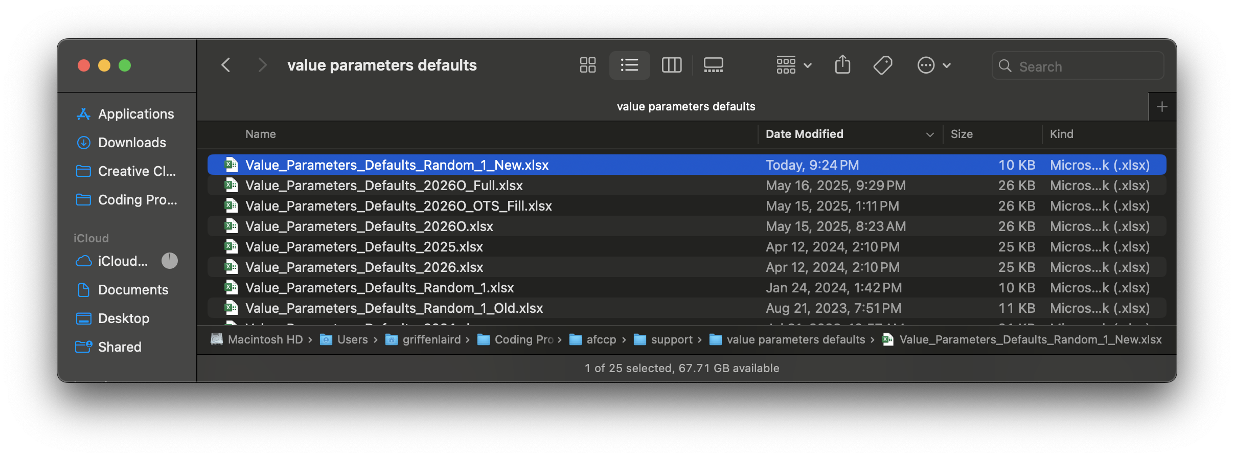
Simply go in and manually change the name to "Value_Parameters_Defaults_Random_1.xlsx" (again, the "New" thing is because I don't want you to accidentally overwrite the real one if applicable!). Once you've done that, we can import this set of value parameters as "defaults" rather than generating random ones like we did at the beginning for this simulated dataset!

v = instance.import_default_value_parameters()  # I add the "v = " because there's a lot of output otherwise

💻 Console Output

Importing default value parameters...
Imported.

There are two reasons I'm having you import the value parameters as defaults above: to show you how can initialize a set of value parameters for an instance from excel (rather than generating random ones), and also to show that I have a nifty function that checks if a new set of value parameters is really "new". What I mean by that is if you acquire a new set of value parameters by importing defaults, ideally it should only be added as a new one if it really is a unique set of parameters. You already had a set of value parameters "VP", and now you've just imported a new one so you should have "VP2". However, you'll still only see "VP" in your list because the two were identical:

# Only one set of value parameters found for this instance
instance.vp_dict.keys()

💻 Console Output

dict_keys(['VP'])

Now that we have our value parameters imported, I want to take a moment to describe the various components. I'm going to do this by using the "Value_Parameters_Defaults" excel file as a reference. Remember, these are the "defaults" that get imported for a particular problem instance that then turn into the actual set of value parameters used. To describe these value parameters, I will show the various dataframes inside the "Value_Parameters_Defaults" excel file structure. This default excel workbook was created when I ran the instance.import_default_value_parameters() method. After changing the name to remove the "_New" extension, I have the file: "support/value parameters defaults/Value_Parameters_Defaults_Random_1.xlsx".

"Overall" value parameters¶

The first dataframe I'll show contains the information for the "big toggles" on the value parameters:

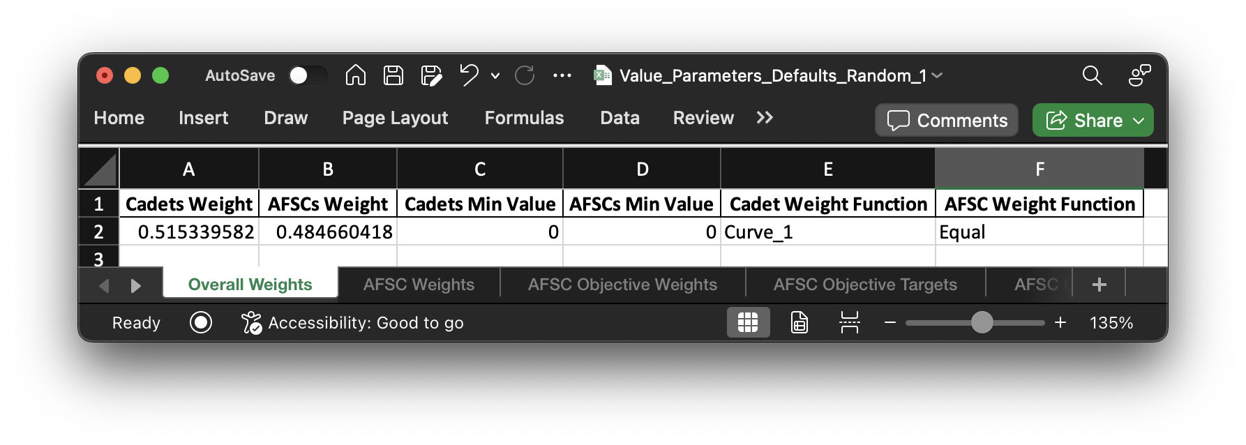
Once initialized for the "Random_1" problem instance, these highest level settings are stored in "Random_1 Value Parameters.csv" in the "Model Input" folder. This dataframe controls the overall settings for each set of value parameters. It's also what tells afccp the names of the different sets of value parameters as well. Right now, we only have one set ("VP").

# Shorthand
p = instance.parameters
vp = instance.value_parameters

print("Current value parameter set name:", instance.vp_name)

# Overall weights on Cadets/AFSCs
print('\nCadets Overall Weight:', vp['cadets_overall_weight'])
print('AFSCs Overall Weight:', vp['afscs_overall_weight'])

# If we want to constrain the overall values on Cadets/AFSCs (we won't, but it's here)
print('\nCadets Overall Minimum Value:', vp['cadets_overall_value_min'])
print('AFSCs Overall Minimum Value:', vp['afscs_overall_value_min'])

💻 Console Output

Current value parameter set name: VP

Cadets Overall Weight: 0.5153395820213456
AFSCs Overall Weight: 0.4846604179786544

Cadets Overall Minimum Value: 0
AFSCs Overall Minimum Value: 0

For the "individual" weight on each cadet relative to all other cadets (and vice versa for AFSCs), we use weight functions. For cadets, their weights are based on their order of merit. In my random set of data, the cadet weight function initialized is "Curve_1". (Yours may differ!)

# Cadet weight function
vp['cadet_weight_function']

💻 Console Output

'Curve_1'

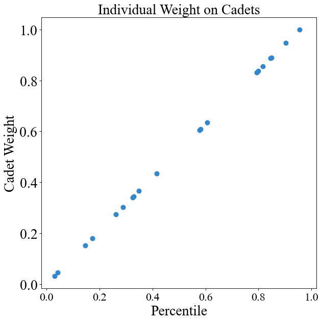
Here, cadet weight is a "sigmoid" function of their order of merit. Again, yours likely will not be! I can illustrate the weight function by plotting cadet weight versus their OM:

chart = instance.display_weight_function({"square_figsize": (8, 8), "dpi": 80})

Now, the percentiles for a real class will be uniformly distributed between 0 and 1. This is a fake class of 20 cadets and so they were randomly selected between 0 and 1 which is why the graph looks a little weird. The y-axis shows the "swing weights" for the cadets. Swing weights simply mean that they've been scaled so the biggest value is 1 and all other weights are relative to that one. "Local" weights, by contrast, sum to 1 collectively. I've printed out the differences below and you can see how I calculate them:

print("Merit", np.around(p['merit'], 3))
print("\n'Local' Weight", np.around(vp['cadet_weight'], 3), "Local Weight Sum:", np.around(np.sum(vp['cadet_weight']), 3))
print("\n'Swing' (Scaled) Weight", np.around(vp['cadet_weight'] / np.max(vp['cadet_weight']), 3))

💻 Console Output

Merit [0.145 0.172 0.288 0.042 0.326 0.329 0.849 0.817 0.349 0.415 0.955 0.031 0.8   0.581 0.794 0.261 0.904 0.578 0.846 0.607]

'Local' Weight [0.026 0.027 0.03  0.026 0.033 0.033 0.074 0.073 0.034 0.04  0.075 0.026 0.073 0.06  0.073 0.029 0.074 0.059 0.074 0.062] Local Weight Sum: 1.0

'Swing' (Scaled) Weight [0.354 0.36  0.408 0.343 0.436 0.438 0.987 0.98  0.457 0.537 1.    0.342 0.975 0.801 0.973 0.392 0.995 0.795 0.987 0.835]

We can also change the weight function through afccp if we want to.

# Linear function of OM (not very "forgiving" to low OM cadets)
instance.change_weight_function(cadets=True, function="Direct")
chart = instance.display_weight_function({"square_figsize": (8, 8), "dpi": 80})

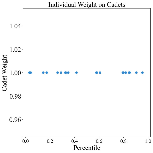
# Cadets are equal no matter what their OM is
instance.change_weight_function(cadets=True, function="Equal")
chart = instance.display_weight_function({"square_figsize": (8, 8), "dpi": 80})

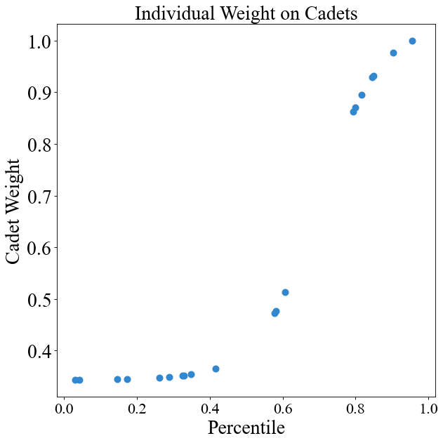
# Exponential curve (not recommended since it puts heavy emphasis on top performers)
instance.change_weight_function(cadets=True, function="Exponential")
chart = instance.display_weight_function({"square_figsize": (8, 8), "dpi": 80})

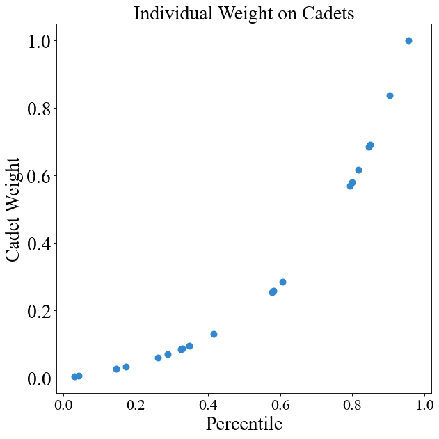
# Sigmoid curve of OM (more forgiving in terms of differences between highest and lowest rank)
instance.change_weight_function(cadets=True, function="Curve_1")
chart = instance.display_weight_function({"square_figsize": (8, 8), "dpi": 80})

These curves are what I'd use since the top cadet is a little more than twice as "important" as the lowest cadet. On the other linear/exponential curves, the difference is quite drastic (100% to 0%).

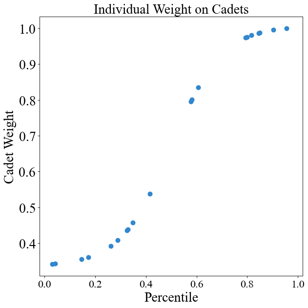
# Sigmoid curve of OM (very similar to previous one)
instance.change_weight_function(cadets=True, function="Curve_2")
chart = instance.display_weight_function({"square_figsize": (8, 8), "dpi": 80})

# Change back to "Curve_1" weight function
instance.change_weight_function(cadets=True, function="Curve_1")
instance.value_parameters['cadet_weight_function']

💻 Console Output

'Curve_1'

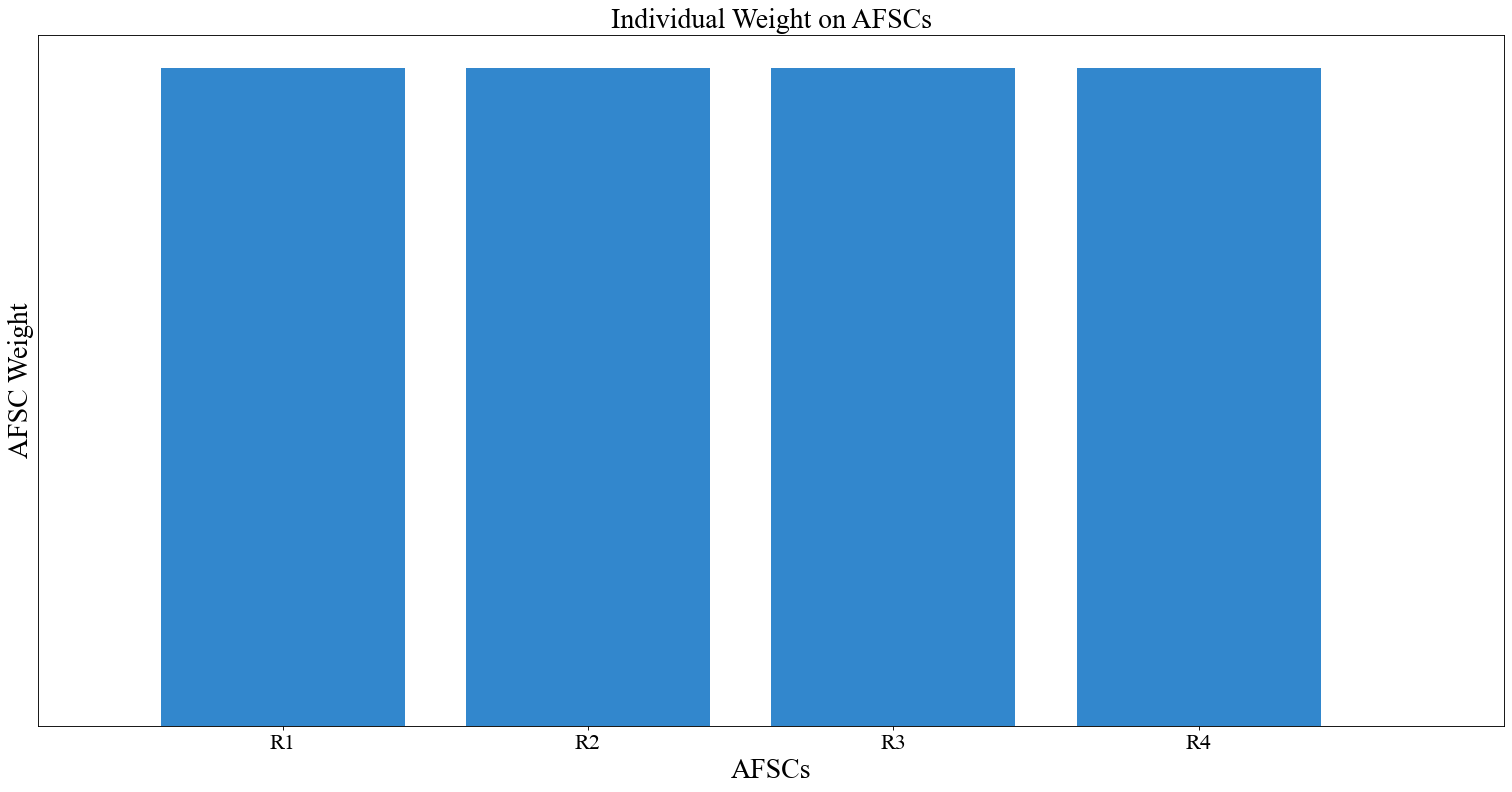
AFSC weights may be determined as a function of their size. Ideally, in the future it'd be some function of their size, difficulty to fill, manpower needs, and maybe more. I want a better method for determining those weights on the AFSCs.

# In my generated data, AFSCs are weighted equally
vp['afsc_weight_function']

💻 Console Output

'Equal'

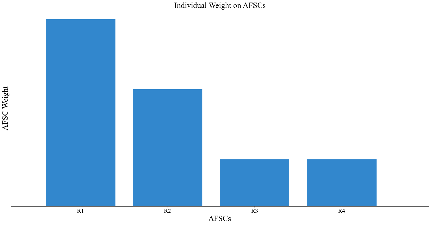
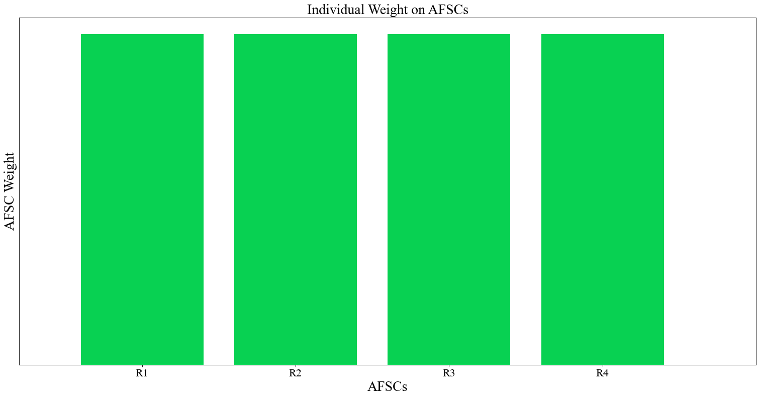
Here is the AFSC weight chart. The AFSC weight chart is a bar chart since we can show relative importance pretty well with those kinds of charts.

chart = instance.display_weight_function(
    {"dpi": 80, "cadets_graph": False, "skip_afscs": False})

# Weight based purely on size
instance.change_weight_function(cadets=False, function="Size")
chart = instance.display_weight_function({"dpi": 80, "cadets_graph": False, "skip_afscs": False})

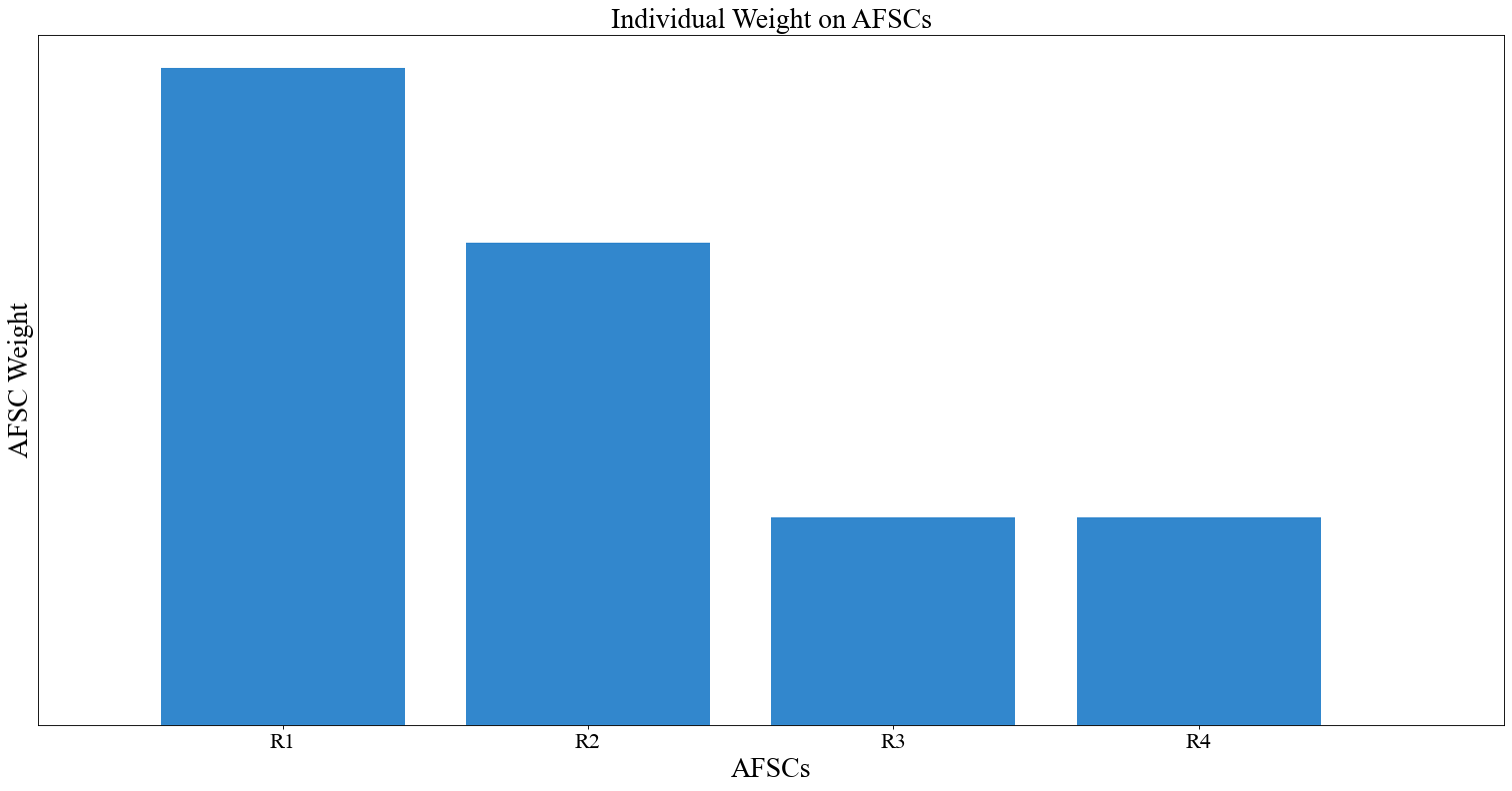
# Slightly different function of size (function from generated data)
instance.change_weight_function(cadets=False, function="Curve_1")
chart = instance.display_weight_function({"dpi": 80, "cadets_graph": False, "skip_afscs": False})

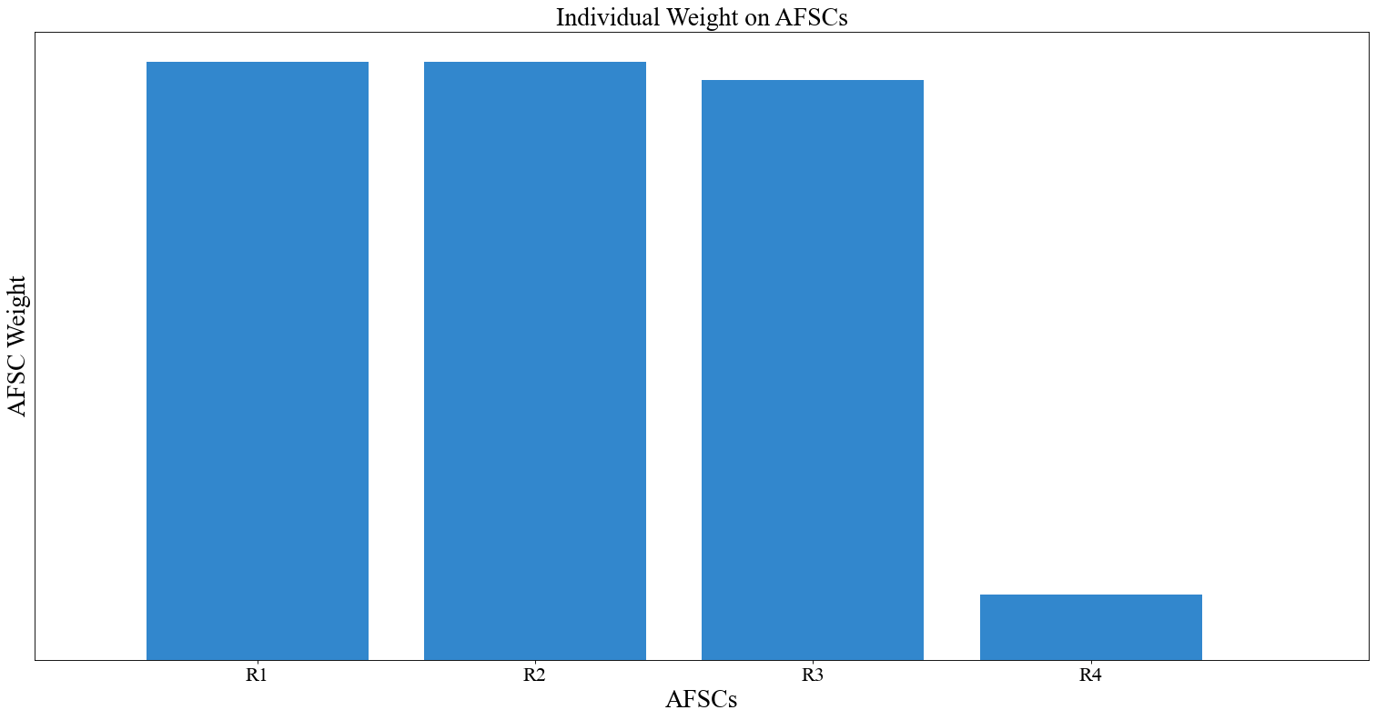
# Another function of size
instance.change_weight_function(cadets=False, function="Curve_2")
chart = instance.display_weight_function({"dpi": 80, "cadets_graph": False, "skip_afscs": False})

# Change back to "Equal" weight function
instance.change_weight_function(cadets=False, function="Equal")
instance.value_parameters['afsc_weight_function']

💻 Console Output

'Equal'

If we pass the function "Custom" for AFSC weights, we will pull from the predefined weights in the "AFSC Weights" excel sheet.

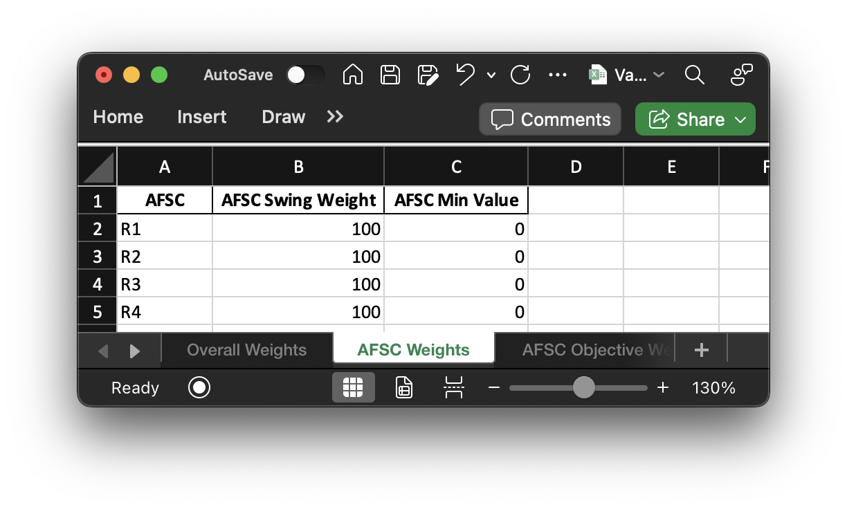
Right now they are from the "Equal" function. If we want to constrain the AFSC values, we can do that using the "AFSC Min Value" column.

print("AFSC 'local' weight:", vp['afsc_weight'])  # Sum to 1!
print("AFSC minimum values:", vp['afsc_value_min'])

💻 Console Output

AFSC 'local' weight: [0.25 0.25 0.25 0.25]
AFSC minimum values: [0. 0. 0. 0.]

I'm going to show the "overall weights" dataset again for reference since there are a lot of charts above and I don't want you to have to keep scrolling up!

I've mentioned the attribute "mdl_p" earlier on in this tutorial but haven't gone too much into detail on it. Essentially, this is my dictionary of all the various toggles and components used across afccp. Everything from genetic algorithm hyperparameters to the colors of various components of the visualizations. There's a lot there. I've actually been using them for the charts above everytime I pass in a dictionary as a parameter for the method I'm calling. If you recall the instance.display_weight_function() method was taking a dictionary including things like {"dpi": 80, "cadets_graph": False, "skip_afscs": False}. These control specific components used in some place within afccp. In that context, they're controls used in the weight function chart.

# DPI (Dots per inch) of my charts
instance.mdl_p['dpi']

💻 Console Output

I alluded to this towards the beginning of the tutorial, but essentially within afccp.core.data.support there is a function called initialize_instance_functional_parameters() that initializes the many "hyperparameters" of afccp. "Hyperparameters" traditionally refer to the parameters that control the learning process of some algorithms and are probably not the best term to use for this since that's really only applicable to the genetic algorithm. "Controls" is probably a better word, since I've generalized this dictionary to control for a lot of different elements. When I say a lot, I mean it!

# Number of keys in the "mdl_p" dictionary
print("Number of afccp 'controls':", len(instance.mdl_p.keys()))

💻 Console Output

Number of afccp 'controls': 246

If you scroll through "main.py" and look at the keyword arguments used you'll notice "p_dict={}" is quite common. What this does is allow you to change the default settings that are initialized for mdl_p. Using "mdl_p" as I do allows me to come up with a needed "control" for some function buried deep within afccp and not worry about passing it through the many layers of functions to get to where it needs to be. The instance object contains mdl_p as an attribute and so we just define it in the parameter initialization function of support.py and bam- we have it wherever we need it. It's also now something I can have a default setting for and potentially change using "p_dict". Here's an example:

# Default bar color- HEX codes are useful ways of selecting precise colors
print('Default bar color:', instance.mdl_p['bar_color'])  # (google "color picker")

💻 Console Output

Default bar color: #3287cd

The color above is the light-ish shade of blue you've seen for the charts above. Let's produce the AFSC chart again after changing the 'bar_color' parameter.

# Slightly different function of size
chart = instance.display_weight_function({"dpi": 80, "cadets_graph": False, "skip_afscs": False, 
                                          'bar_color': "#08d152"})  # Shade of green

As a reminder, in order to make use of p_dict as a means of passing a new value for one of the controls inside "mdl_p", you simply call the desired method and pass a dictionary ie. {"bar_color": "blue"} containing the keys that you want to change as the only argument.

AFSC Objectives¶

Before I dive deep into the components of the AFSC objectives, it's probably worthwhile to talk about what the objectives themselves are. Here they are printed out for you:

vp['objectives']

💻 Console Output

array(['Norm Score', 'Merit', 'USAFA Proportion', 'Combined Quota',
   'USAFA Quota', 'ROTC Quota', 'Utility', 'Mandatory', 'Desired',
   'Permitted', 'Tier 1', 'Tier 2', 'Tier 3', 'Tier 4'], dtype='<U16')

The "Norm Score" objective refers to the newly defined career field preference lists. Basically, career fields get to rank cadets in order of preference similar to how the cadets rank their AFSC choices. To evaluate how well we meet the needs of the AFSC according to their preferences, I came up with a normalized score idea. Imagine you have a set of ten cadets, ranked 1 to 10. If you are picking 3 cadets from that list, the best cadets you could select are the ones ranked 1, 2, 3. The worst are the cadets ranked 8, 9, 10. The former is a score of 1 and the latter is a score of 0. Whatever you ultimately pick is likely going to be somewhere in between, which is where the norm score comes in. Here is that example:

import random

# Cadet rankings
num_cadets = 10  # 10 cadets in the above example
rankings = np.arange(num_cadets) + 1
print('Rankings:', rankings)

# Picking "n" cadets
n = 3  # picking 3 for this example

# Selecting n cadets
print('\nBest Cadets:', rankings[:n])

# "Score" is the sum of these numbers
best_score = np.sum(rankings[:n])
print('Best Cadets Score:', best_score)

# Selecting n cadets
print('\nWorst Cadets:', rankings[num_cadets-n:])

# "Score" is the sum of these numbers
worst_score = np.sum(rankings[num_cadets-n:])
print('Worst Cadets Score:', worst_score)

# Pick a random set of n cadets
selected_cadets = random.sample(list(rankings), n)
print('\nRandomly selected cadets:', selected_cadets)

selected_score = np.sum(selected_cadets)
print('Random cadets score:', selected_score)

# "Norm Score" normalizes that "selected_score" on a 1 to 0 scale using the best/worst scores
norm_score = 1 - (selected_score - best_score) / (worst_score - best_score)
print('\nNorm Score:', round(norm_score, 4))

# Everything described above is what is used in afccp
from afccp.solutions.handling import calculate_afsc_norm_score_general

# This function takes the rankings and selected rankings as arguments
norm_score_2 = calculate_afsc_norm_score_general(rankings, selected_cadets)  
print('Norm Score (from afccp):', round(norm_score_2, 4))

💻 Console Output

Rankings: [ 1  2  3  4  5  6  7  8  9 10]

Best Cadets: [1 2 3]
Best Cadets Score: 6

Worst Cadets: [ 8  9 10]
Worst Cadets Score: 27

Randomly selected cadets: [10, 4, 8]
Random cadets score: 22

Norm Score: 0.2381
Norm Score (from afccp): 0.2381

The "Merit" objective is one that was used to fairly distribute "quality" cadets across the AFSCs. The idea is that no single "large" AFSC should be composed of entirely high or low performers. I've never liked this objective because it puts too much emphasis on defining quality for a career field purely on graduating order of merit. I believe that the career field preferences provide a much better way of defining quality cadets that is specific to each career field. It is no longer a zero-sum game, and it is theoretically possible (though highly improbable) that the rankings given could perfectly line up with the needs of the Air Force such that every single AFSC receives their top performers. Again, this won't ever happen, but we are now deviating from order of merit as the one-size-fits-all metric of quality.

# Average order of merit of the class
print('Average OM:', np.mean(p['merit'])) # Should be about 0.5 for a real class (random data will not)

# Proportion of USAFA cadets of the class
print('USAFA Proportion:', np.mean(p['usafa'])) # Closer to 1/3 for a real class

💻 Console Output

Average OM: 0.5044154990687344
USAFA Proportion: 0.35

In a very similar way that we want to keep average OM around 0.5 (or whatever the actual average is) for each of the large AFSCs, we also don't want any single large AFSC to be composed of entirely USAFA or ROTC cadets. We take the actual proportion of the cadets as the baseline and then shoot to be within +- 15% of that number. That is another AFSC objective that may or may not actually be that important. The idea now is that it should be left up to the career field manager to determine.

# USAFA quota (for each AFSC)
print('USAFA Quota:', p['usafa_quota'])

# ROTC quota (for each AFSC)
print('ROTC Quota:', p['rotc_quota'])

💻 Console Output

USAFA Quota: [1. 1. 0. 0.]
ROTC Quota: [7. 4. 2. 2.]

If you recall the USAFA/ROTC quotas from earlier on, these numbers are fed into their appropriate objectives. Meeting the individual USAFA and ROTC quotas are two objectives that are separate from the USAFA proportion objective. They're doing similar things, but one is trying to balance the proportion of cadets assigned to be around some baseline while the others are simply trying to meet a quota and that's it. These objectives really only come into play now with the rated AFSCs since we need to keep the slots specific to each source of commissioning.

# The "desired" number of cadets for a given AFSC
print('PGL Target (Combined SOC quotas):', p['pgl'])
print('\nDesired number:', p['quota_d'])

💻 Console Output

PGL Target (Combined SOC quotas): [8. 5. 2. 2.]

Desired number: [8. 8. 3. 2.]

The quota objective that we absolutely do care about is the "Combined Quota" objective which is used right now to meet the PGL. It currently provides the minimum number of cadets to classify and so as long as we meet each of the minimums then we are good! In the future, there's a lot more we should do with this objective to really hone in on the importance of assigning more or fewer cadets to a given AFSC (cross-collaboration with AFMAA/A1XD in the works).

# The AFOCD Tier objectives (from the "AFSCs.csv" I showed earlier)
p['Deg Tiers']

💻 Console Output

array([['M > 0.27', 'P < 0.73', '', ''],
       ['P = 1', 'I = 0', '', ''],
       ['M = 1', 'I = 0', '', ''],
       ['P = 1', 'I = 0', '', '']], dtype='<U8')

There are generally up to four Air Force Officer Classification Directory (AFOCD) degree tiers per career field. Each degree tier has a target proportion and requirement level associated with it: Mandatory, Desired, or Permitted (M, D, P). Above, the columns correspond to degree tiers (1, 2, 3, 4) and the rows are the AFSCs. It just so happens that in this example we have 4 AFSCs and so it's worth clarifying! The format above provides a few pieces of information: the requirement level, target proportion, and the type of inequality specified (>, <, or =). So, for a degree tier format of "D > 0.54", we know the requirement is "Desired" and the AFSC wants at LEAST 54% of their accessions to have degrees in that tier. If you recall, the information on what tier everyone is placed in for each AFSC based on their degree is located in the "qual" matrix. There is a function in afccp.core.support called cip_to_qual_tiers() that creates the qual matrix based on the cadets' degrees. This is an important function for the AFPC/DSYA analyst to maintain, and is irrelevant for random data since it's all fake anyway!

# Qual matrix! This conveys requirement level (M, D, P), tier (1, 2, 3, 4) and even eligibility ("I" is ineligible)
p['qual']  # Rows are cadets, columns are AFSCs!

💻 Console Output

array([['M1', 'P1', 'I2', 'P1'],
       ['M1', 'P1', 'I2', 'P1'],
       ['P2', 'P1', 'M1', 'P1'],
       ['P2', 'P1', 'M1', 'I2'],
       ['M1', 'I2', 'I2', 'P1'],
       ['P2', 'P1', 'M1', 'P1'],
       ['P2', 'P1', 'M1', 'I2'],
       ['M1', 'P1', 'M1', 'P1'],
       ['M1', 'P1', 'I2', 'P1'],
       ['P2', 'I2', 'M1', 'P1'],
       ['M1', 'I2', 'I2', 'P1'],
       ['P2', 'P1', 'I2', 'P1'],
       ['P2', 'P1', 'M1', 'P1'],
       ['M1', 'I2', 'M1', 'I2'],
       ['M1', 'P1', 'I2', 'P1'],
       ['P2', 'P1', 'M1', 'I2'],
       ['P2', 'P1', 'M1', 'P1'],
       ['P2', 'P1', 'M1', 'P1'],
       ['P2', 'P1', 'M1', 'P1'],
       ['P2', 'P1', 'M1', 'P1']], dtype='<U2')

As you can imagine, the objectives for "Tier 1" -> "Tier 4" are there to meet the respective degree tier proportions! There are the legacy "Mandatory", "Desired", and "Permitted" objectives as well, but those were replaced with the tier objectives ("Tier 1" -> "Tier 4"). Essentially, we used to just group each of the categories (M, D, P) together and constrain the model that way. This was not completely accurate, since two tiers that both have a mandatory label (M) should be treated separately.

Lastly, the "Utility" objective is simply to maximize cadet utility (happiness) and is measured by the average cadet utility of the cadets assigned. I have this in there so AFSCs can prioritize the preferences of their incoming cadets as well.

AFSC Objective Components¶

This section describes the various pieces of the AFSC objectives: their weights, targets, and constraints. The value functions are another component of the objectives, but we'll cover them in their own section since there's a lot going on there! The first component of the AFSC objectives we'll discuss are the weights.

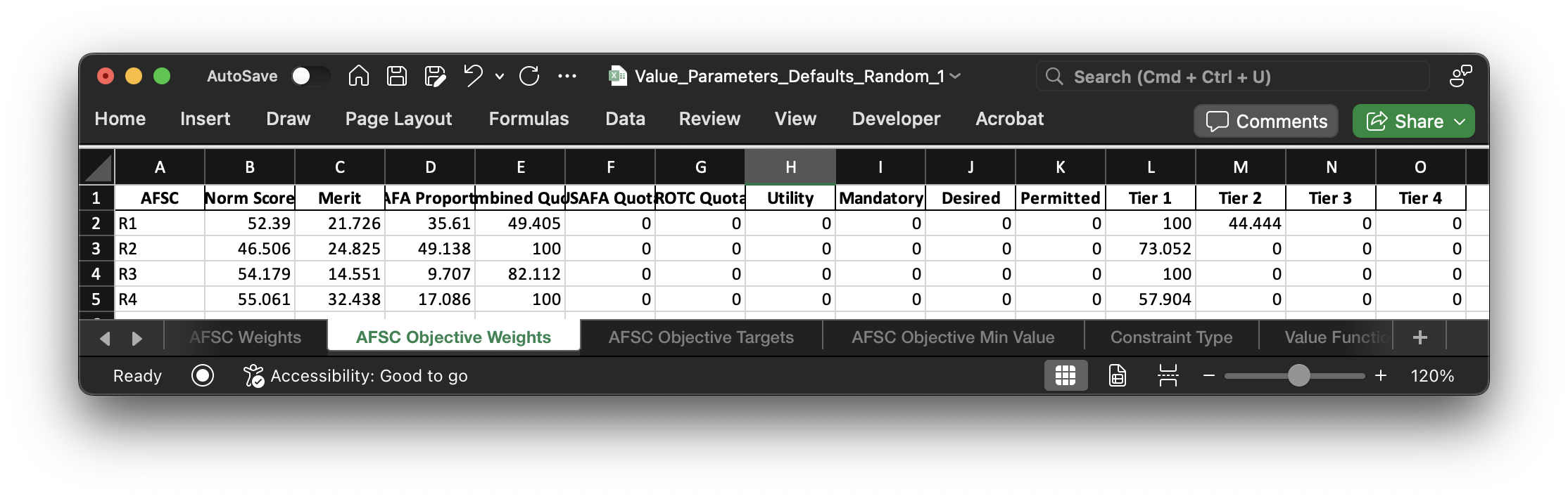
Here are the objective weights for each AFSC for each objective. Like the AFSC "individual" weights, these are swing weights that will be scaled for each AFSC so that they sum to 1. Many objectives are weighted at 0 which effectively removes them from consideration for a given AFSC.

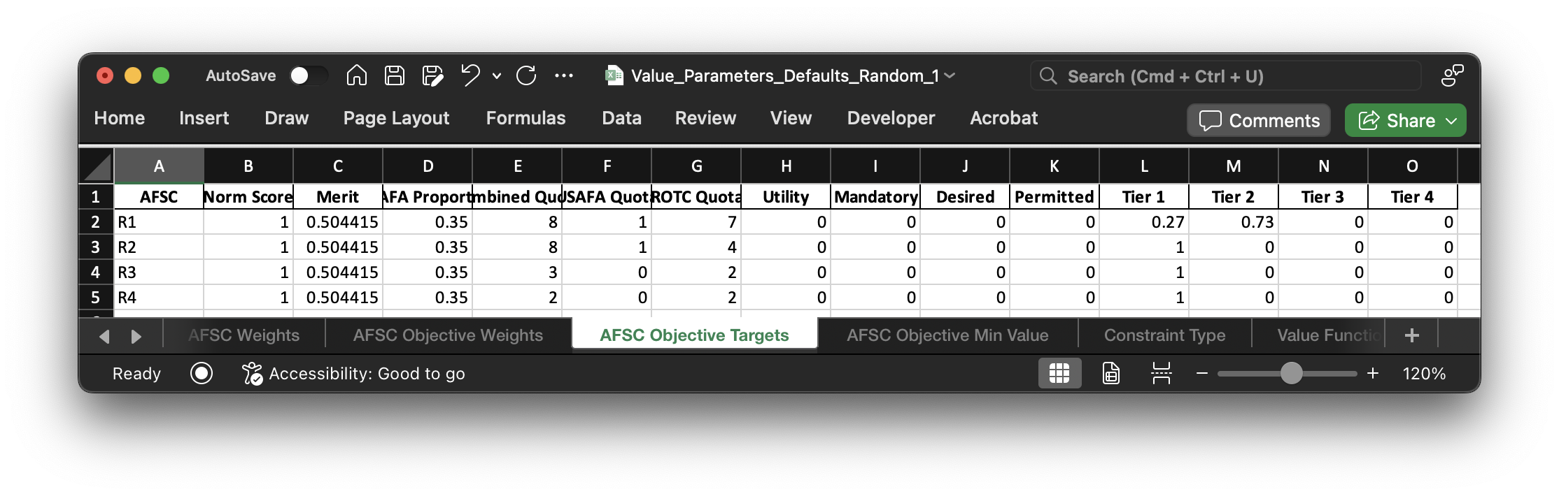
This dataframe displays the target measure for each of the objectives. In a perfect world, we'd meet every AFSC objective by hitting these values for each of them.

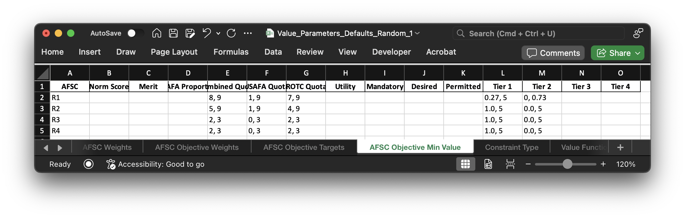
These are the constraints for each objective for each AFSC. Most are determined automatically based on the "fixed" data. For example, the Combined Quota constraint is determined by the "Min, Max" values in "Random_1 AFSCs.csv". The AFOCD Tier objective constraint ranges come from the "Deg Tiers" columns of "Random_1 AFSCs.csv" as well. Since this is random data, nothing else is constrained to begin with.

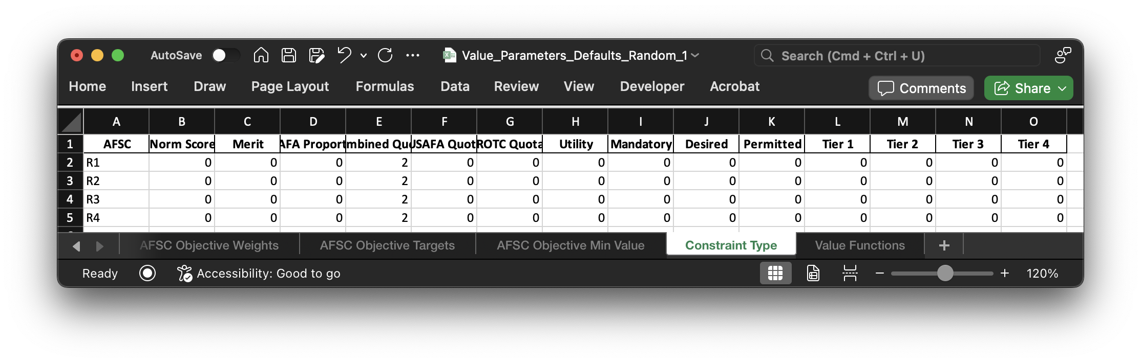
Here is where you actually turn different constraints on or off. If there is a 0, the constraint is turned off. A "1" is an "approximate" constraint. This means that the denominator is the PGL target for an AFSC, not the actual number of cadets assigned. If this is confusing, please reference my thesis or my slides that talk about the difference between the Approximate Model and the Exact Model. The "2", therefore, is an "exact" constraint. The only place where we could legitimately use a "1" instead of a "2" is for the AFOCD constraints.

Example: Let's say 14N wants 70% of their cadets to have tier 1 degrees. Let's also say the PGL is 190 and we assign 220 cadets. A "1" constraint is a less restrictive constraint, and would ensure that 133 cadets (190 * 0.70) have "Tier 1" degrees. Alternatively, a "2" constraint ensures the actual proportion gets constrained, so 154 cadets (220 * 0.70) will have "Tier 1" degrees. Sometimes it is really hard to meet the AFOCD for some AFSCs, and so a "1" constraint is necessary to ensure we meet the target based on the PGL, not the actual number of cadets. Most of the time, however, we use "2" as the constraint type.

Once these default value parameters have been imported/initialized for Random_1, they will be imported from "Random_1 VP.csv" in "Model Input".

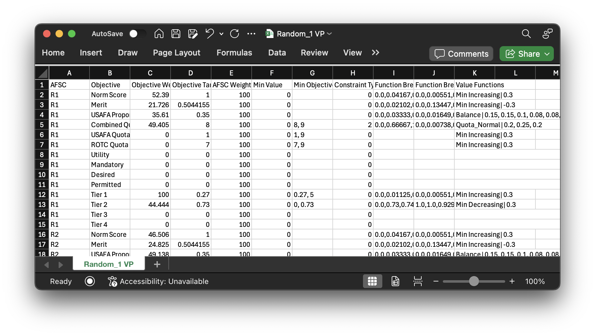
As you can see, this file structure has a row for every AFSC and objective pair. The dataframes shown previously are flattened into columns and exist here. Again, these are the actual value parameters used for the problem instance, since the "Defaults" could have been more generalized (they aren't here since we exported our randomly generated set as defaults, therefore having it be the same thing as what you're seeing here). For a real class you could simply take the previous years defaults, tweak them a bit if needed, and import those as a starting point for a new class year. The objective targets would be updated to reflect the information of the problem instance you're looking at (the USAFA proportion objective target would be the proportion of the USAFA cadets of the instance you're solving, for example).

The "AFSC Weight" and "Min Value" columns above pertain to the AFSC itself, not the AFSC-objective pair like the others (which is why "AFSC Weight" is all 100s for R1). The three columns to the right pertain to the value functions used for each AFSC and objective which I will discuss in more detail in the following section.

Value Functions¶

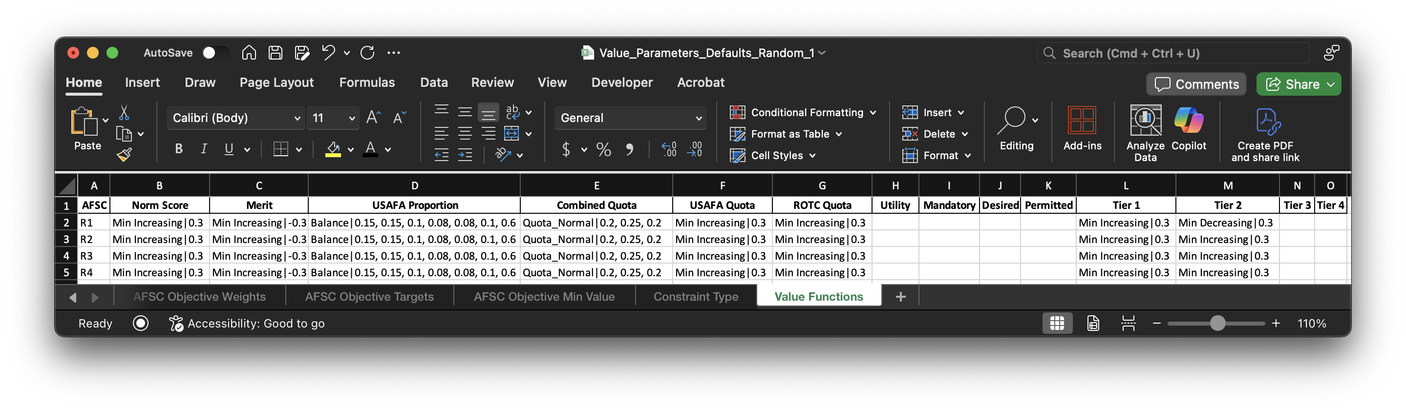
Here we have the value functions for each of the AFSC objectives. These definitely require some explaining. I've created my own terminology so that they can be generalized and constructed into actual value functions for each of the objectives. I have an excel file that outlines how these functions are created and what they look like (Value_Function_Builds.xlsx), but I will also detail them here.

# I need to import this script
import afccp.data.values

Before you read this next section on the value functions, please look at my "Creating Value Functions" slides in VFT_Model_Slides.pptx (starts on slide 130), and just click through them. This is how I construct the value functions, and this should help your understanding of the different piece-wise "segments" used.

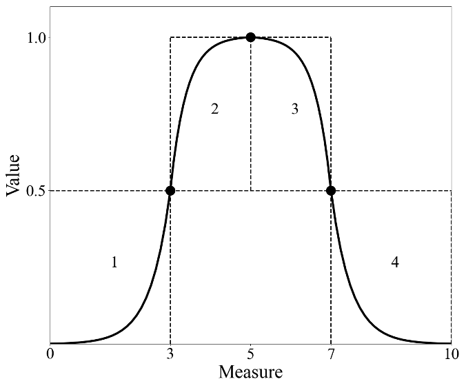
The purpose of the "vf_string" (Value Function string) is to construct the "segment_dict" (Segment Dictionary) which provides the coordinates for the main piece-wise value function segment breakpoints. As illustrated below, there are four "segments" of exponential functions that are pieced together using "breakpoints". There are therefore 5 breakpoints. For this example, they are at the coordinates (0, 0), (3, 0.5), (5, 1), (7, 0.5), and (10, 0). This would compose the "segment_dict".

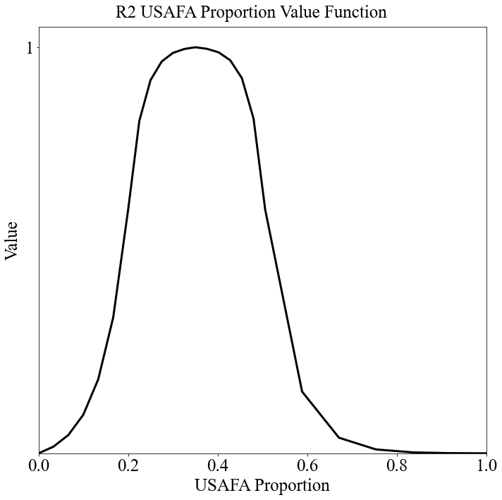
Let's illustrate the "Balance" value function. It takes several inputs pertaining to the "margins" and the \(\rho\) parameters. Here is what it looks like:

vf_string \(=\) "Balance|left_base_margin, right_base_margin, \(\rho_1\), \(\rho_2\), \(\rho_3\), \(\rho_4\), margin_y"

Honestly, you really don't need to worry about what these all mean. The only thing you should focus on is the \(\rho\) ("rho") parameters. These control how steep each of the exponential segments are. Let's see an example. We'll first generate the "segment_dict" based on the "vf_string":

vf_string = "Balance|0.2, 0.2, 0.1, 0.08, 0.08, 0.1, 0.5"
target = 0.5
actual = 0.5
segment_dict = afccp.data.values.create_segment_dict_from_string(vf_string, target=target, actual=actual)
for segment in segment_dict:
    print(str(segment) + ":", segment_dict[segment])

💻 Console Output

1: {'x1': 0, 'y1': 0, 'x2': 0.3, 'y2': 0.5, 'rho': -0.1}
2: {'x1': 0.3, 'y1': 0.5, 'x2': 0.5, 'y2': 1, 'rho': 0.08}
3: {'x1': 0.5, 'y1': 1, 'x2': 0.7, 'y2': 0.5, 'rho': 0.08}
4: {'x1': 0.7, 'y1': 0.5, 'x2': 1, 'y2': 0, 'rho': -0.1}

Now we have our segment dictionary! We know what the coordinates for the "main" breakpoints are, so we can now generate the rest of the breakpoints to make the function linear. Let's calculate the x and y coordinates of our function's breakpoints.

x, y = afccp.data.values.value_function_builder(segment_dict=segment_dict, num_breakpoints=20)
print("x:", x, "\n\n", "y:", y)

💻 Console Output

x: [0.   0.06 0.12 0.18 0.24 0.3  0.34 0.38 0.42 0.46 0.5  0.54 0.58 0.62 0.66 0.7  0.76 0.82 0.88 0.94 1.  ] 

y: [0.      0.00288 0.01245 0.04423 0.14973 0.5     0.8182  0.93527 0.97833 0.99417 1.      0.99417 0.97833 
    0.93527 0.8182  0.5     0.14973 0.04423 0.01245 0.00288 0.     ]

Now we plot our value function!

# "Balance" type of value function!
from afccp.visualizations.charts import ValueFunctionChart
chart = ValueFunctionChart(x, y)

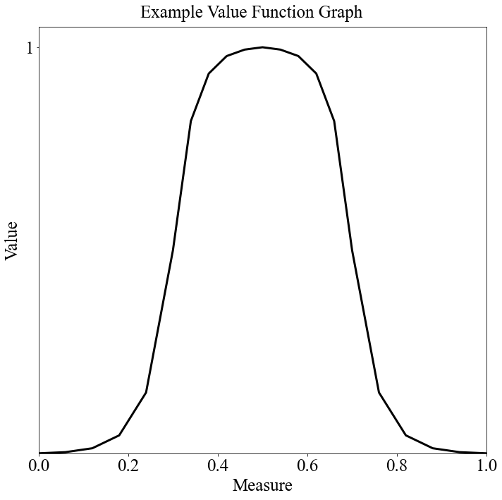
And there we have it. This is the value function we've constructed from that initial "vf_string". Play around with the different parameters and see what happens here!

# Change this
vf_string = "Balance|0.2, 0.2, 0.1, 0.08, 0.08, 0.1, 0.5"
target = 0.5  # This is what we're after
actual = 0.5  # This is essentially what we could realistically expect (based on set of eligible cadets)
num_breakpoints = 200  # How many breakpoints to use 
# (the more breakpoints used, the more the function appears non-linear)

# Don't change this
segment_dict = afccp.data.values.create_segment_dict_from_string(vf_string, target=target, actual=actual)
x, y = afccp.data.values.value_function_builder(segment_dict=segment_dict, num_breakpoints=num_breakpoints)
chart = ValueFunctionChart(x, y)

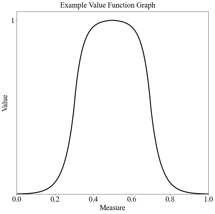
That is the "Balance" value function type. This is intended for the objectives that seek to "balance" certain characteristics of the cadets (USAFA proportions and sometimes Merit as well). I did end up changing the Merit value function to be a "Min Increasing" because I decided against penalizing the objective for exceeding 0.5. At this point, I will note that these value functions don't necessarily have to have 4 segments. I do have value function types that use 3, 2, or even 1 segment. Let's discuss the quota value functions.

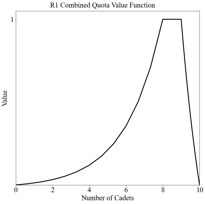
"Quota_Direct" is intended for AFSCs that have a range on the number of cadets that are to be assigned, but also know around where they'd like to fall within that range. There are 6 parameters, the \(\rho\) (rho) parameters for each of the four segments, and the y values for the two breakpoints on either side of the "peak". The vf_string is then: "Quota_Direct|\(\rho_1\), \(\rho_2\), \(\rho_3\), \(\rho_4\), \(y_1\), \(y_2\)". The additional AFSC specific parameters are the upper/lower bounds on the number of cadets as well as the actual target number of cadets within that range. Here is an example:

vf_string = "Quota_Direct|0.1, 1, 0.6, 0.1, 0.8, 0.8"
minimum = 120  # Lower Bound
maximum = 200  # Upper Bound
target = 140  # Desired number of cadets within the range
num_breakpoints = 200  # How many breakpoints to use 

# Don't change this
segment_dict = afccp.data.values.create_segment_dict_from_string(vf_string, target=target, 
                                                                      minimum=minimum, maximum=maximum)
x, y = afccp.data.values.value_function_builder(segment_dict=segment_dict, num_breakpoints=num_breakpoints)
chart = ValueFunctionChart(x, y)

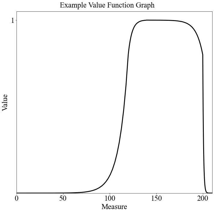
Here you can see that although the range of 120 to 200 is specified, there is a direction of preference within that range (the AFSC wants around 140 cadets, but is fairly accepting of values around that range). I will note that the target, minimum, and maximum parameters are taken from the "Random_1 AFSCs.csv" data!

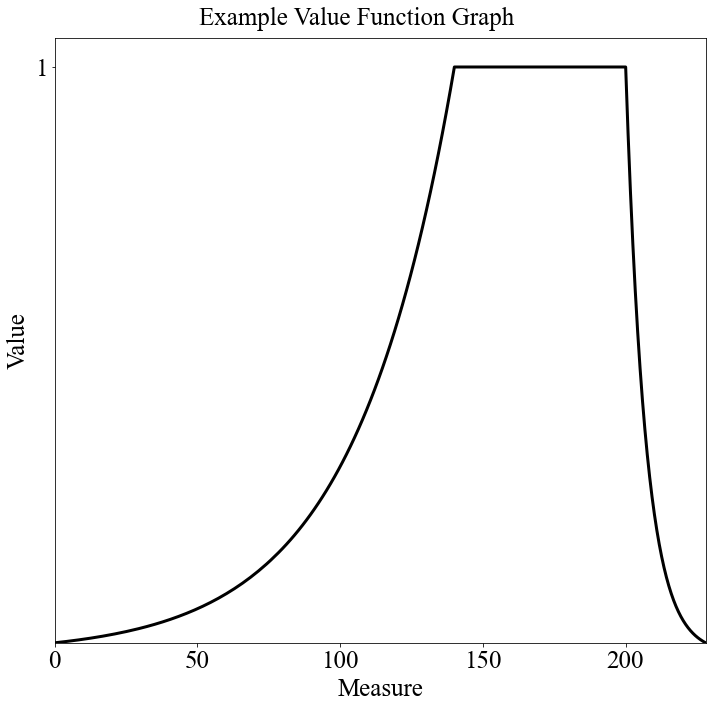
Another value function we can choose for the quota objective is the "Quota_Normal" function type. This is intended for AFSCs that either don't care about the number of cadets (as long as they fall within a certain range) or didn't specify. For example, the PGL says 120 and after speaking with them we determine the upper bound is 200 and they say they have no preference between 120 and 200 and everything in between. There are 2 segments for this function, connected by a horizontal line at y = 1 for the range on the cadets. The function parameters are \(\rho_1\), \(\rho_2\), and "domain_max" which is the max number of cadets that could have a nonzero value (arbitrary scalar just to get a curve on the right side of the function). Here is the vf_string: "Quota_Normal|d_max, \(\rho_1\), \(\rho_2\)". Here is an example:

vf_string = "Quota_Normal|0.2, 0.25, 0.05"
minimum = 120  # Lower Bound
maximum = 200  # Upper Bound
target = 140  # (Doesn't matter here)
num_breakpoints = 200  # How many breakpoints to use 

# Don't change this
segment_dict = afccp.data.values.create_segment_dict_from_string(vf_string, target=target, 
                                                                      minimum=minimum, maximum=maximum)
x, y = afccp.data.values.value_function_builder(segment_dict=segment_dict, num_breakpoints=num_breakpoints)
chart = ValueFunctionChart(x, y)

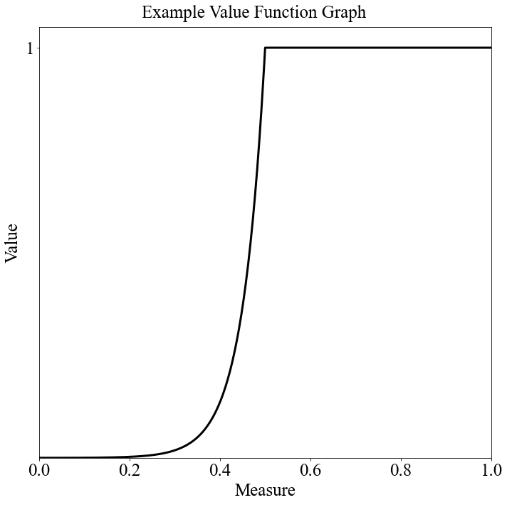
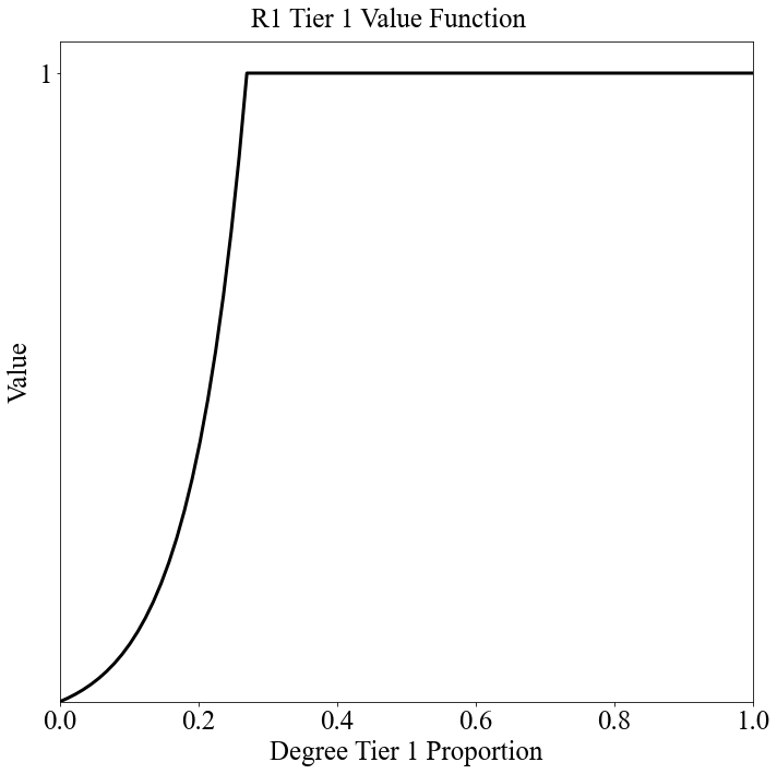
The last two kinds of value functions I'll discuss are the "Min Increasing" and "Min Decreasing" types. They are very simple and only have one segment which is a simple exponentional curve to get to the target measure (in the x space). The only parameter is \(\rho\). The vf_string then looks like: "Min Increasing|\(\rho\)" or "Min Decreasing|\(\rho\)". They are called "Min" functions because it's essentially the same thing as taking the minimum value between some exponential curve and 1. Here are some examples:

vf_string = "Min Increasing|0.1"
target = 0.5
num_breakpoints = 200  # How many breakpoints to use 

# Don't change this
segment_dict = afccp.data.values.create_segment_dict_from_string(vf_string, target=target)
x, y = afccp.data.values.value_function_builder(segment_dict=segment_dict, num_breakpoints=num_breakpoints)
chart = ValueFunctionChart(x, y)

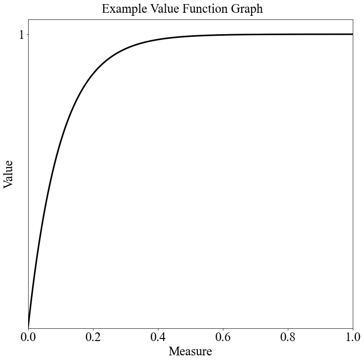
vf_string = "Min Increasing|-0.1"
target = 1
num_breakpoints = 200  # How many breakpoints to use 

# Don't change this
segment_dict = afccp.data.values.create_segment_dict_from_string(vf_string, target=target)
x, y = afccp.data.values.value_function_builder(segment_dict=segment_dict, num_breakpoints=num_breakpoints)
chart = ValueFunctionChart(x, y)

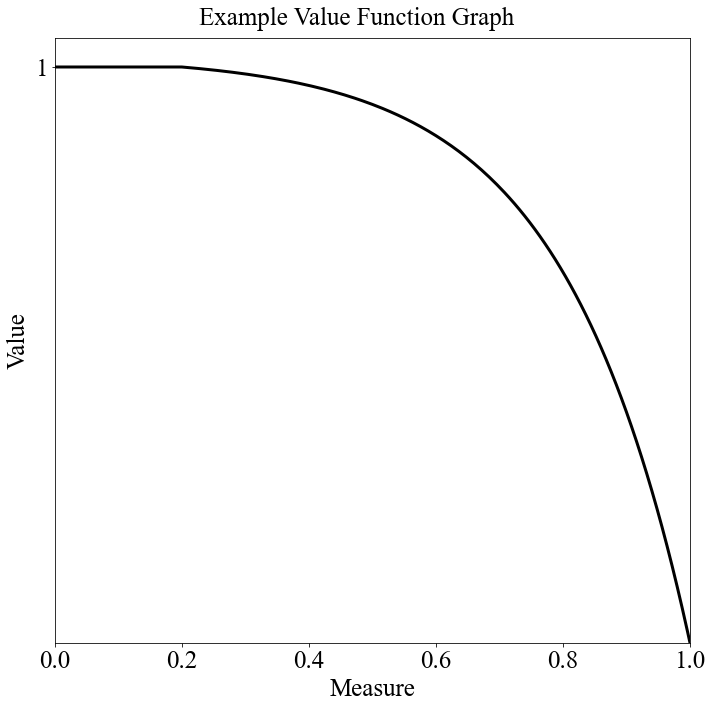
vf_string = "Min Decreasing|-1"
target = 0.2
num_breakpoints = 200  # How many breakpoints to use 

# Don't change this
segment_dict = afccp.data.values.create_segment_dict_from_string(vf_string, target=target)
x, y = afccp.data.values.value_function_builder(segment_dict=segment_dict, num_breakpoints=num_breakpoints)
chart = ValueFunctionChart(x, y)

vf_string = "Min Decreasing|1"
target = 0.2
num_breakpoints = 200  # How many breakpoints to use 

# Don't change this
segment_dict = afccp.data.values.create_segment_dict_from_string(vf_string, target=target)
x, y = afccp.data.values.value_function_builder(segment_dict=segment_dict, num_breakpoints=num_breakpoints)
chart = ValueFunctionChart(x, y)

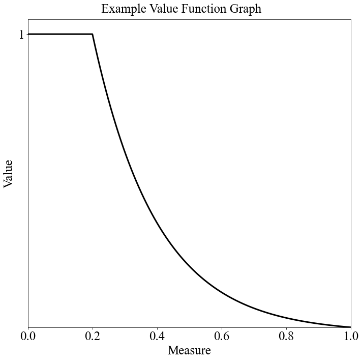
And there you have it! This is how I code up and construct my many value functions for each of the objectives for each of the AFSCs. Please reach out if you have any questions as I know this is a confusing section.

Now that we're done discussing the types of value functions, we can take a look at the actual value functions used on "Random_1". We're plotting the breakpoints (x/y coordinates) for a specific AFSC objective value function. Here is an example:

# Plot the value function (this also saves it to the "Value Functions" sub-folder by default FYI)
c = instance.show_value_function({'afsc': "R1", 'objective': 'Combined Quota'})

💻 Console Output

Creating value function chart for objective Combined Quota for AFSC R1

# Plot the value function (this also saves it to the "Value Functions" sub-folder by default FYI)
c = instance.show_value_function({'afsc': "R2", 'objective': 'USAFA Proportion'})

💻 Console Output

Creating value function chart for objective USAFA Proportion for AFSC R2

# Plot the value function (this also saves it to the "Value Functions" sub-folder by default FYI)
c = instance.show_value_function({'afsc': "R1", 'objective': 'Tier 1'})

💻 Console Output

Creating value function chart for objective Tier 1 for AFSC R1

Global Utility¶

There are a few other components of the "value parameters" that I haven't mentioned yet. The global_utility matrix is based on the cadets' preferences as well as the AFSCs' preferences. The two matrices cadet_utility and afsc_utility are merged according to the overall weights on the cadets/AFSCs.

# Cadet Utility Matrix
p['cadet_utility']  # As a reminder 'p' -> 'instance.parameters'!!!

💻 Console Output

array([[1.    , 0.4683, 0.    , 0.1917],
       [1.    , 0.5433, 0.    , 0.3667],
       [0.135 , 1.    , 0.42  , 0.65  ],
       [0.7933, 0.4717, 1.    , 0.    ],
       [1.    , 0.    , 0.    , 0.355 ],
       [1.    , 0.2   , 0.47  , 0.805 ],
       [0.7133, 1.    , 0.1817, 0.    ],
       [1.    , 0.21  , 0.42  , 0.655 ],
       [1.    , 0.3833, 0.    , 0.1767],
       [0.1867, 0.    , 1.    , 0.3633],
       [0.265 , 0.    , 0.    , 1.    ],
       [1.    , 0.7983, 0.    , 0.3917],
       [0.645 , 0.495 , 1.    , 0.325 ],
       [1.    , 0.    , 0.43  , 0.    ],
       [0.8083, 1.    , 0.    , 0.3467],
       [0.7233, 0.4217, 1.    , 0.    ],
       [0.355 , 0.2   , 1.    , 0.5   ],
       [0.855 , 0.72  , 1.    , 0.52  ],
       [1.    , 0.56  , 0.21  , 0.725 ],
       [0.29  , 0.135 , 0.66  , 1.    ]])

# AFSC Utility Matrix
p['afsc_utility']

💻 Console Output

array([[0.75      , 0.0625    , 0.        , 0.0625    ],
       [0.6       , 0.25      , 0.        , 0.3125    ],
       [0.05      , 0.6875    , 0.07692308, 0.4375    ],
       [0.2       , 0.3125    , 0.23076923, 0.        ],
       [0.55      , 0.        , 0.        , 0.375     ],
       [0.4       , 0.1875    , 0.15384615, 0.5       ],
       [0.7       , 0.9375    , 0.38461538, 0.        ],
       [1.        , 0.5625    , 0.69230769, 0.8125    ],
       [0.45      , 0.125     , 0.        , 0.125     ],
       [0.1       , 0.        , 0.76923077, 0.25      ],
       [0.85      , 0.        , 0.        , 1.        ],
       [0.25      , 0.5       , 0.        , 0.1875    ],
       [0.5       , 0.75      , 0.92307692, 0.6875    ],
       [0.9       , 0.        , 0.30769231, 0.        ],
       [0.95      , 1.        , 0.        , 0.5625    ],
       [0.3       , 0.4375    , 0.53846154, 0.        ],
       [0.35      , 0.625     , 1.        , 0.625     ],
       [0.65      , 0.8125    , 0.84615385, 0.75      ],
       [0.8       , 0.875     , 0.46153846, 0.9375    ],
       [0.15      , 0.375     , 0.61538462, 0.875     ]])

# Overall weights on cadets/AFSCs
print("weight on cadets:", round(vp['cadets_overall_weight'], 2))
print("weight on AFSCs:", round(vp['afscs_overall_weight'], 2))

💻 Console Output

weight on cadets: 0.52
weight on AFSCs: 0.48

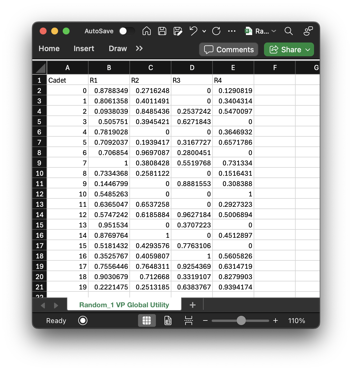
# Global Utility Matrix (Each cell is the weighted sum of cadet/AFSC utility)
vp['global_utility']  # Extra column is for the unmatched cadets!

💻 Console Output

array([[0.8788349 , 0.2716248 , 0.        , 0.12908187, 0.        ],
       [0.80613583, 0.4011491 , 0.        , 0.34043141, 0.        ],
       [0.09380386, 0.84854362, 0.2537242 , 0.54700966, 0.        ],
       [0.50575097, 0.39454206, 0.62718429, 0.        , 0.        ],
       [0.78190281, 0.        , 0.        , 0.36469321, 0.        ],
       [0.70920375, 0.19394174, 0.31677274, 0.65717857, 0.        ],
       [0.70685402, 0.96970872, 0.28004506, 0.        , 0.        ],
       [1.        , 0.3808428 , 0.55197676, 0.73133402, 0.        ],
       [0.73343677, 0.25811221, 0.        , 0.15164306, 0.        ],
       [0.14467994, 0.        , 0.88815529, 0.30838797, 0.        ],
       [0.54852634, 0.        , 0.        , 1.        , 0.        ],
       [0.63650469, 0.6537258 , 0.        , 0.29273234, 0.        ],
       [0.57472424, 0.61858841, 0.96271843, 0.5006894 , 0.        ],
       [0.95153396, 0.        , 0.3707223 , 0.        , 0.        ],
       [0.87697638, 1.        , 0.        , 0.45128972, 0.        ],
       [0.51814325, 0.42935763, 0.77631058, 0.        , 0.        ],
       [0.3525767 , 0.40598068, 1.        , 0.56058255, 0.        ],
       [0.75564461, 0.76483109, 0.92543686, 0.6314719 , 0.        ],
       [0.90306792, 0.71266803, 0.33191074, 0.82799034, 0.        ],
       [0.22214754, 0.2513185 , 0.63837669, 0.93941745, 0.        ]])

print("Cadet 0's utility on AFSC 0:", p['cadet_utility'][0, 0])
print("AFSC 0's utility on cadet 0:", p['afsc_utility'][0, 0])
print("Global Utility[0, 0]:", round(vp['cadets_overall_weight'], 2), "*", p['cadet_utility'][0, 0], "+", 
     round(vp['afscs_overall_weight'], 2), "*", p['afsc_utility'][0, 0], "=", vp['global_utility'][0, 0])

💻 Console Output

Cadet 0's utility on AFSC 0: 1.0
AFSC 0's utility on cadet 0: 0.75
Global Utility[0, 0]: 0.52 * 1.0 + 0.48 * 0.75 = 0.8788348955053363

The global utility matrix is unique to each set of value parameters (since you can toggle the weights on cadets/AFSCs and get a different matrix). This matrix lives in "Random_1 VP Global Utility.csv":

Cadet Utility Constraints (Meant just for AFPC/DSYA through an operational lens)¶

Another component of the value parameters is the cadet utility constraints. These constraints ensure certain cadets receive some minimum utility value, and the implication here usually applies to the top 10% of cadets as my method of preventing as much of the "adjudication" piece on the backend. Built into the classification process is adjudication where the sources of commissioning get to review the results prior to release and make adjustments as needed. One thing they always want to make sure is that their top cadets are getting something they want, and if they aren't they'll kick it back to AFPC to fix. I can use the cadet utility constraints to ensure that the top 10% of cadets receive one of their top 3 choices, or there is a good reason why they aren't getting one (if they only have very competitive AFSCs as their top 3 choices and don't rank high enough for them then that may cause problems).

These constraints live in the file "Random_1 Cadets Utility Constraints.csv":

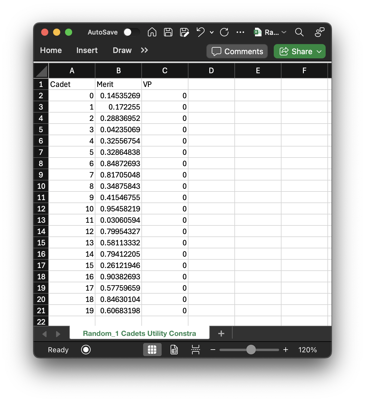
As you can see, I include the cadet indices (as I've said before, it's because I like referring to cadets by their indices in the numpy arrays since that allows me to do a lot of things) as well as the cadets' order of merit. This information gives more context to why certain cadets have constrained minimum values versus other cadets! The "VP" column is the actual constrained minimum utilities for all the cadets. If you have a second set of value parameters that you're using, there would be another column called "VP2". As you can see, the default is to keep all the cadets unconstrained. I've thought a lot about how this should work and wrestled with the idea of just making a function to go through and constrain the top 10% to get a utility value greater than or equal to their third choice but ultimately decided against it. The reason is that it's more complicated than that, and I firmly believe the AFPC/DSYA analyst needs to be the one to do it manually.

When I ran this for FY23 and FY24, I tuned the model parameters to be what I needed them to be based on everyone's wants and desires and then solved it initially without any cadet constraints. I can then look at the solution at the top 10/20% of the class and if the cadet is receiving a top 3 preference anyway (vast majority do), then I constrain their utilities to be whatever their third choice utility was. I then filter on the people who aren't getting a top 3 preference. If the reason is just because the optimal solution involved this cadet not getting a top 3 preference, and they really should have received one based on preferences (they didn't have 3 very hard choices to meet), then I also enforce the utility constraint. If there's a clear reason why they're getting their fourth choice (and I mean a VERY justifiable reason), then I constrain them to their fourth choice utility. For top 10%, I don't think this happened at all but did occur for top 20%.

# Cadet utility constriants
vp['cadet_value_min']  # Defaults to 0! For an example problem (not real class year), don't mess with this

💻 Console Output

array([0., 0., 0., 0., 0., 0., 0., 0., 0., 0., 0., 0., 0., 0., 0., 0., 0.,
       0., 0., 0.])

Goal-Programming Parameters¶

One final input file that I haven't mentioned is "Random_1 Goal Programming.csv". These are the inputs that another AFIT researcher, former Lt. Rebecca Reynolds (now Capt. Rebecca Eisemann), used for her goal-programming model. My intent for afccp has always been to provide a way for researchers in this field to contribute to this "academic" problem and try new things to inspire innovation for AFPC/DSYA. For her goal programming model, her inputs are structured in this way:

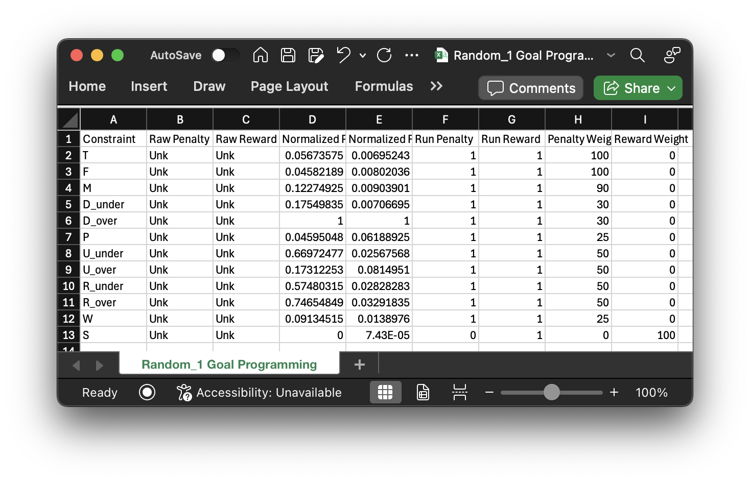
In order to get the penalty/reward terms here we need to run the model on the specific class year to tune the parameters to get the actual parameters needed to run the full goal programming model. It's a little nuanced and you can certainly view her thesis here. I will briefly cover her model a little more later on.

📌 Summary¶

This tutorial explains how to generate and customize value parameters for cadet-to-AFSC matching within the AFCCP model. Value parameters are central to the Value-Focused Thinking model through the use of modeling AFSC objectives. That said, since the main model used now is the GUO model, most of the contents of the value_parameters dictionary are no longer used. That said, there are still some components that are very much used (like the constraints).

The tutorial walks through:

Default Value Generation
How to use predefined "defaults" to create baseline value parameters.
AFSC Objectives and Components The data available for each AFSC and objective (weights, targets, constraints, value functions)
Custom Curve Generation
Methods to create and visualize alternative value functions using exponential or polynomial interpolation.
Adjustments and Additions
How to modify value curves for specific AFSCs or cadet groups, including smoothing and parameter additions.
Visualization
Optional plotting functions to help understand the shape and effect of each value function.

By the end, you should have a fully defined set of value_parameters stored in the appropriate dictionary structure to feed into the various afccp optimization models. You’re now ready to continue on and discover the data methods used to correct the parameters in Tutorial 5!

Tutorial 4: Value Parameters¶

Defaults¶

"Overall" value parameters¶

Model Controls ("mdl_p" side-bar)¶

AFSC Objectives¶

AFSC Objective Components¶

Value Functions¶

Global Utility¶

Cadet Utility Constraints (Meant just for AFPC/DSYA through an operational lens)¶

Goal-Programming Parameters¶

📌 Summary¶