Tutorial 6: Solutions Overview

As you've seen, afccp requires a substantial amount of data in order to work. All the various parameters, v alue parameters, hyper-parameters, and other "controls" are necessary to determine the best solution assignment of cadets to AFSCs. This is the whole point of afccp: obtain the right solution! This section of the tutorial contains the information needed for you to calculate different solutions through various algorithms and models.

solutions Module

The solutions module of afccp contains the scripts and functions that handle the determination of a solution assignment of cadets to AFSCs. Each script tackles solutions in a different way. At a high-level, the module is set up as follows:

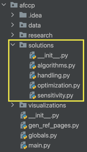
The algorithms module contains the matching algorithms, SOC algorithms, and meta-heuristics that solve this problem. This is meant to contain all the non-optimization solvers for the problem. Alternatively, optimization contains the optimization models formulated using the python optimization library pyomo. Pyomo is a great library that seamlessly links native python language with optimization components. The sensitivity module incorporates the optimization models to allow for a more algorithmic approach to solving them. We can iterate through different parameters and solve the models accordingly to provide interesting data perspectives to help inform why the solution is the way it is. Lastly, handling contains the many functions that all involve handling and processing the different solutions that are generated. We need to be able to evaluate these solutions and come up with key metrics that are used to determine which one to implement.

Structure

Before we dive into the different methods of generating a solution, it's important to discuss what exactly a solution is, or rather how a solution is represented, in the context of afccp. In the same way that the parameters (data) can all be extracted from csvs and pulled into python dictionaries, the solutions for a given instance are also pulled from csvs into a python dictionary. This is where the instance sub-folder "5. Analysis & Results" plays a role.

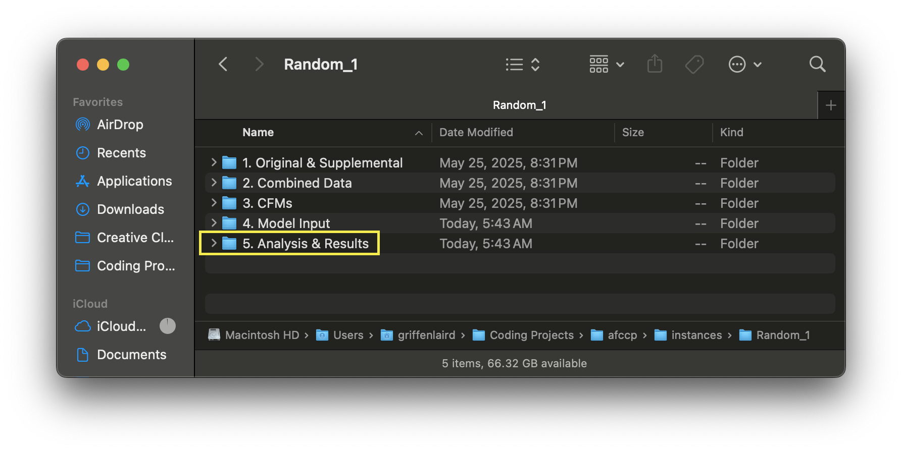
When working with the CadetCareerProblem object, several sub-folders of this folder will be created that hold many of the visualizations you may be working with. One of the different controls (mdl_p) is the dictionary key "save" which determines whether we should save charts that are created back to your folders. It is defaulted to True which means that there will be some charts saved into some of these sub-folders already, assuming that you've been following along with your own code.

As mentioned previously, we use dictionaries to hold solutions and solution elements. There are two instance attributes that contain this information: "solution" and "solutions". The first, "solution", is a dictionary containing all the components and metrics of the current activated solution. In the same way that we activate a particular set of value_parameters, we also activate a particular solution to analyze for the problem. The second attribute "solutions" is a dictionary of solution dictionaries. The keys are the names of each solution and the values are that particular solution's component dictionary. Confusing, yes, but it will hopefully be made clear soon.

# Re-import Random_1 instance
instance = CadetCareerProblem('Random_1')
instance.set_value_parameters()
instance.update_value_parameters()
instance.parameter_sanity_check()
print('')  # Add buffer between print statements

# Showing that there currently are no solutions available to this "Random_1" instance
print("Current activated solution (instance.solution):", instance.solution)
print("Current set of solutions (instance.solutions):", instance.solutions)

💻 Console Output

Importing 'Random_1' instance...
Instance 'Random_1' initialized.
Sanity checking the instance parameters...
Done, 0 issues found.

Current activated solution (instance.solution): None
Current set of solutions (instance.solutions): None

We have not yet created any solutions, so none will appear in the "Analysis & Results" folder either. Let's start by creating a random solution and then exporting it back to excel as an example.

# Generate random solution
instance.generate_random_solution()

# Export all data back to excel
instance.export_data()

💻 Console Output

Generating random solution...
New Solution Evaluated.
Measured exact VFT objective value: 0.4947.
Global Utility Score: 0.4245. 0 / 0 AFSCs fixed. 0 / 0 AFSCs reserved. 0 / 0 alternate list scenarios respected.
Blocking pairs: 19. Unmatched cadets: 0.
Matched cadets: 20/20. N^Match: 20. Ineligible cadets: 0.

Exporting datasets ['Cadets', 'AFSCs', 'Preferences', 'Goal Programming', 'Value Parameters', 'Solutions', 'Additional', 'Base Solutions', 'Course Solutions']

If you now look at your Analysis & Results folder, you should have a csv file titled "Random_1 Solutions.csv". This dataset contains a column for the cadet indices (0 through 19 in our case) accompanied by the solution columns themselves. There could be as many solution columns as desired stored within this dataset. Right now, we have one solution "Random" containing an assortment of randomly selected AFSCs for each cadet.

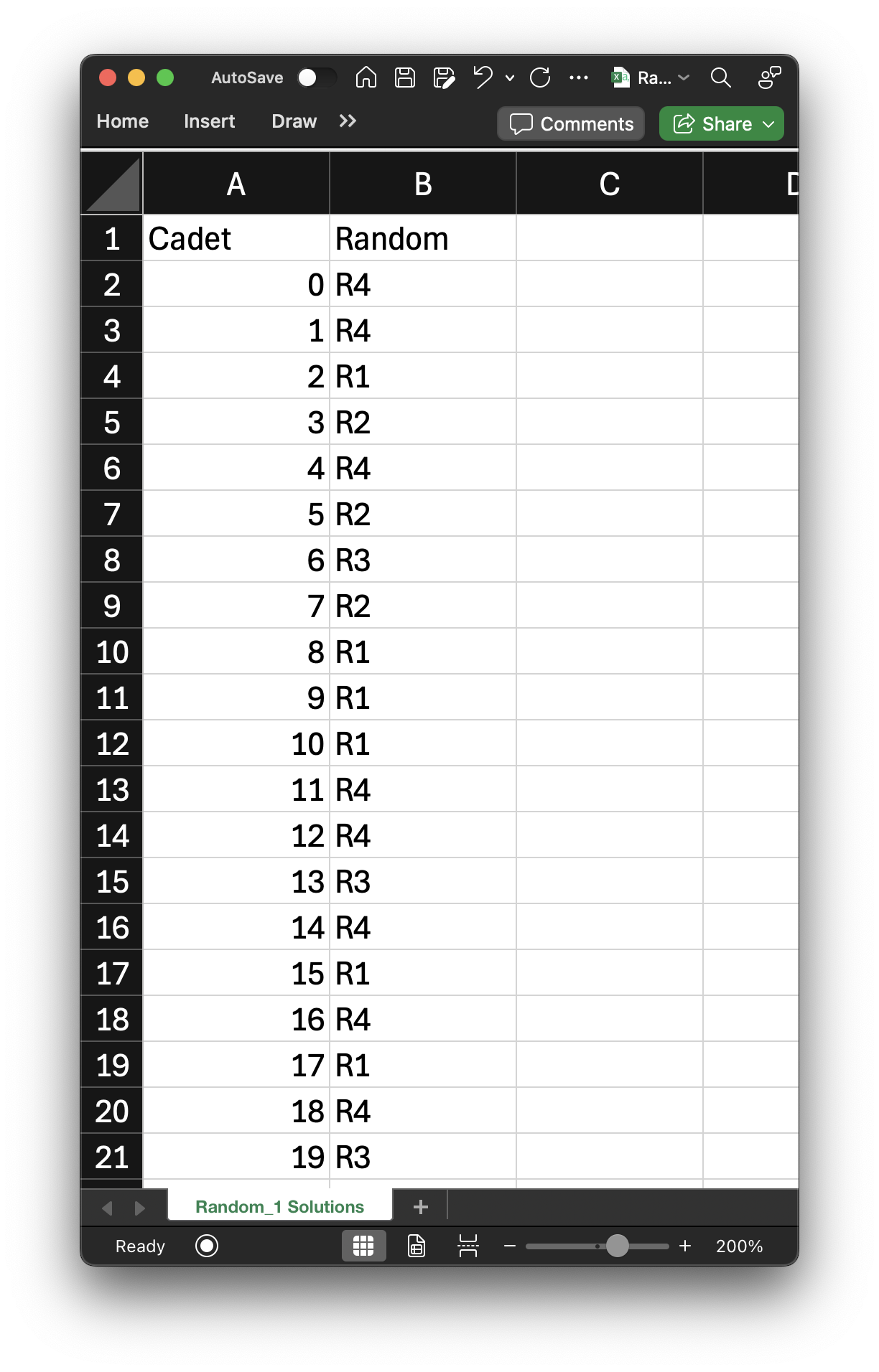
A couple of notes: This is a picture of my randomly generated solution and won't match your output (it's random, after all)! Additionally, don't confuse the solution name "Random" with the instance name "Random_1". We're dealing with a randomly generated problem instance of cadets/AFSCs, and now we've just introduced our first method of generating a solution: "Random"! These are two different random components. Let's now "start over" and re-import the Random_1 problem instance, so we can see how this solution is initially stored in the CadetCareerProblem object.

# Re-import "Random_1"
instance = CadetCareerProblem("Random_1")

# "Activate" a particular set of value parameters (since you can have multiple)
instance.set_value_parameters("VP")  # There could be "VP", "VP2", "VP3", etc.

# In case you change some parameter that the value parameters depend on
instance.update_value_parameters()  # AFSC quotas are a good example here

# Always make sure your data is good to go!
instance.parameter_sanity_check()

💻 Console Output

Importing 'Random_1' instance...
Instance 'Random_1' initialized.
Sanity checking the instance parameters...
Done, 0 issues found.

To hopefully highlight the good practices of working with afccp, I've included the other methods I recommend to have on here after you import a dataset. This instance now has solution data stored in the Analysis & Results folder, which is contained in the instance attribute "solutions". We have not "activated" a solution, however.

# Showing the names of the solutions we currently have
print("Names of solutions:", instance.solutions.keys())

# Contents of the "Random" solution
print("'Random' solution components:", instance.solutions['Random'].keys())

# Current solution (haven't selected it yet)
print("Current activated solution components:", instance.solution)

💻 Console Output

Names of solutions: dict_keys(['Random'])
'Random' solution components: dict_keys(['j_array', 'name', 'afsc_array'])
Current activated solution components: None

You might be wondering why I don't just automatically select "Random" as the current solution. When you're doing this for the real thing, you'll likely be dealing with multiple solutions, and I want you to be sure you know which solution you're dealing with. That's why I force the analyst to select a specific solution.

# Select the "Random" solution (just like the value parameters)
instance.set_solution("Random")  # By default, the first solution is selected if no name is provided

# Current solution
print("\nCurrent activated solution components (first 5):", list(instance.solution.keys())[:5])

# Number of solution components (after evaluating the solution)
print("Number of solution components:", len(instance.solution.keys()))

💻 Console Output

Solution Evaluated: Random.
Measured exact VFT objective value: 0.4947.
Global Utility Score: 0.4245. 0 / 0 AFSCs fixed. 0 / 0 AFSCs reserved. 0 / 0 alternate list scenarios respected.
Blocking pairs: 19. Unmatched cadets: 0.
Matched cadets: 20/20. N^Match: 20. Ineligible cadets: 0.


Current activated solution components (first 5): ['j_array', 'name', 'afsc_array', 'x', 'objective_measure']
Number of solution components: 76

When you activate a solution, or generate one for that matter, afccp also evaluates it according to the parameters of the instance. This is what's happening for the first several lines of output above (before my explicit print statements). The functions that do this live in afccp.solutions.handling, which I highly encourage you to explore especially if you're thinking about tracking your own metrics (I already have a lot of them calculated there!). These metrics then get placed into the solution dictionary, and I've printed the first 5 keys of that dictionary above. I also highlight the reason I'm only printing the first five by including the total number of solution dictionary keys right below that!

# Name of the solution
print("Name of solution ('name'):", instance.solution['name'])

# Array of AFSC names that each cadet is assigned to
print("\nAFSC names that each cadet is assigned ('afsc_array'):", instance.solution['afsc_array'])

# Array of AFSC indices that each cadet is assigned to
print("\nAFSC indices that each cadet is assigned ('j_array'):", instance.solution['j_array'])

# Binary X-matrix where the rows are cadets and columns are AFSCs
print("\nX-Matrix ('x'):\n", instance.solution['x'])

💻 Console Output

Name of solution ('name'): Random

AFSC names that each cadet is assigned ('afsc_array'): ['R4' 'R4' 'R1' 'R2' 'R4' 'R2' 'R3' 'R2' 'R1' 'R1' 'R1' 'R4' 'R4' 'R3'
 'R4' 'R1' 'R4' 'R1' 'R4' 'R3']

AFSC indices that each cadet is assigned ('j_array'): [3 3 0 1 3 1 2 1 0 0 0 3 3 2 3 0 3 0 3 2]

X-Matrix ('x'):
 [[0 0 0 1]
 [0 0 0 1]
 [1 0 0 0]
 [0 1 0 0]
 [0 0 0 1]
 [0 1 0 0]
 [0 0 1 0]
 [0 1 0 0]
 [1 0 0 0]
 [1 0 0 0]
 [1 0 0 0]
 [0 0 0 1]
 [0 0 0 1]
 [0 0 1 0]
 [0 0 0 1]
 [1 0 0 0]
 [0 0 0 1]
 [1 0 0 0]
 [0 0 0 1]
 [0 0 1 0]]

As you can probably tell "afsc_array", "j_array", and "x" all contain the same information just presented in three different ways. The "afsc_array" is what is ultimately stored in the "Solutions.csv" file because of its ease of interpretability. The "x" matrix is what optimization models output, and it is how the solution is evaluated according to the VFT objective hierarchy (which I will describe later). By far my preferred method of representing a solution, which is used almost everywhere across afccp (outside the two cases I just described), is "j_array". Utilizing the power of numpy indexing allows us to quickly and efficiently extract necessary information from "j_array".

# Array of cadets assigned to each AFSC stored in a dictionary
{j: np.where(instance.solution['j_array'] == j)[0] for j in instance.parameters['J']}

💻 Console Output

{0: array([ 2,  8,  9, 10, 15, 17]),
 1: array([3, 5, 7]),
 2: array([ 6, 13, 19]),
 3: array([ 0,  1,  4, 11, 12, 14, 16, 18])}

I use numpy.where() extensively across afccp, and the above line of code is an example of why I like using indices. By the way, the above information is already incorporated in the solution dictionary (see below).

# Array of cadets assigned to each AFSC stored in the "cadets_assigned" component
instance.solution['cadets_assigned']

💻 Console Output

{0: array([ 2,  8,  9, 10, 15, 17]),
 1: array([3, 5, 7]),
 2: array([ 6, 13, 19]),
 3: array([ 0,  1,  4, 11, 12, 14, 16, 18])}

For more information on what specifically the code currently tracks, I again invite you to look at the functions in afccp.solutions.handling. Specifically, the evaluate_solution function is the main function that obtains this information.

The convention I use when determining solution names is to incorporate both the solution method and iteration. The only method I've discussed thus far is "Random", which is why the current solution is called "Random". I've only generated one random solution too. By default, the first solution you generate through whatever method will simply be named using that method. If I were to generate a second solution, it would be called "Random_2" (see below).

# Generate another random solution
instance.generate_random_solution()

# Current activated solution name
print("\nCurrent activated solution name:", instance.solution['name'])

# Current solutions available
print("Curretn solutions available:", instance.solutions.keys())

💻 Console Output

Generating random solution...
New Solution Evaluated.
Measured exact VFT objective value: 0.5456.
Global Utility Score: 0.588. 0 / 0 AFSCs fixed. 0 / 0 AFSCs reserved. 0 / 0 alternate list scenarios respected.
Blocking pairs: 13. Unmatched cadets: 0.
Matched cadets: 20/20. N^Match: 20. Ineligible cadets: 0.


Current activated solution name: Random_2
Curretn solutions available: dict_keys(['Random', 'Random_2'])

In the same way I check if a set of value parameters is unique, I also make sure a new solution is unique too. There is a very low probability that two randomly generated solutions are the same, but if that did happen we wouldn't see a "Random_2" solution above. Instead, the code would simply kick back the "Random" solution as the current solution since it is equivalent to the new one. This does play a critical role with the deterministic models/algorithms you will see soon as I don't want many copies of the same solution being depicted as unique.

📌 Summary

Tutorial 6 introduces how the afccp framework handles solutions—the assignment of cadets to AFSCs based on value parameters, optimization criteria, and algorithmic controls. It explains the structure of the solutions module within afccp, which includes submodules for algorithms, optimization, sensitivity analysis, and solution handling.

The tutorial guides you through:

• Generating random solutions and exporting them to Excel.
• Understanding the format of solution dictionaries (solution and solutions) and their components.
• Activating and evaluating a solution using the CadetCareerProblem object.
• Comparing different solution representations: afsc_array, j_array, and the binary assignment matrix x.
• Exploring how metrics and analytics (like blocking pairs and global utility) are computed and stored.
• Naming conventions and uniqueness checks for solutions.

You also learn about the role of the "5. Analysis & Results" folder for storing evaluated outputs and how to inspect solution quality programmatically. Continue on to Tutorial 7 to dive into the algorithms & meta-heuristics of afccp.